Diffusion Equation: a computational approach
computational physics, applied math, probability
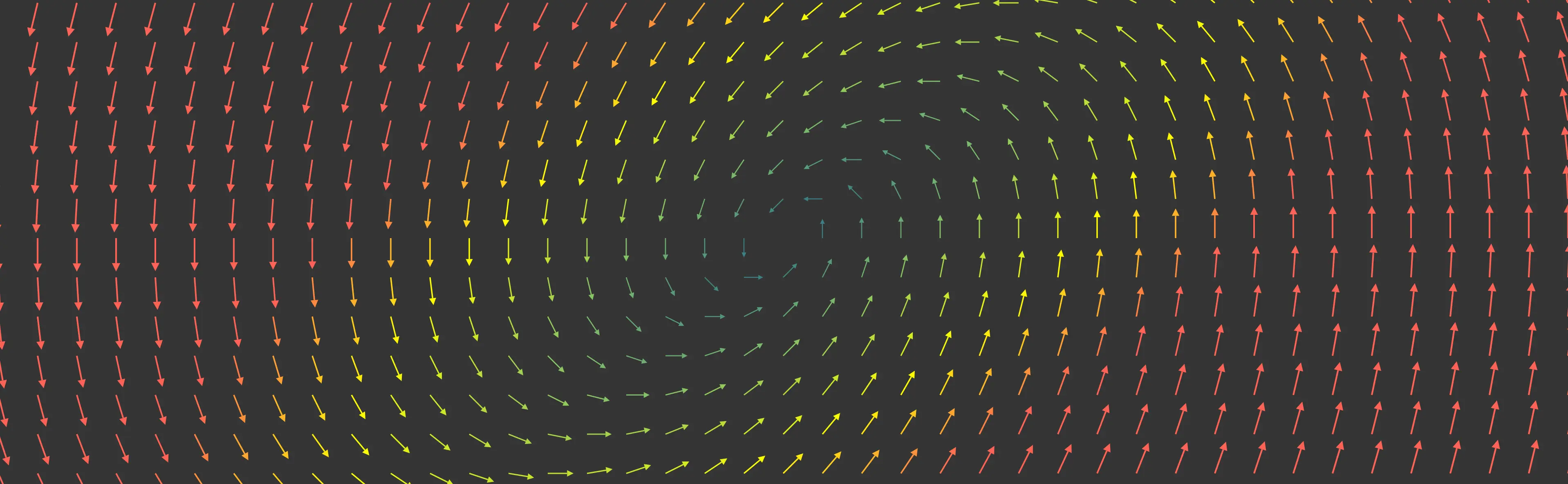
Table of Contents
Prerequisites
- High school calculus or beyond
- Probability
- Some basic physics.
Motivation
Recently, I have been watching The Office TV show. In one of the episodes named “Lice”, Dwight Schrute (The assistant to the Regional Manager) had an insecticidal grenade, and he hilariously dropped it, and immediately the smoke diffused all over the place. The scene looked a bit fake; however, the way the smoke spread was a kind of catchy, so I had to figure out what is going around.

Background
Convection-Diffusion Equation , generally, describes a transfer of physical quantities like energy (commonly heat), or particles within a physical system. Depending on the nature of the application, we can tweak the equation a little bit, or even omit some terms when we seek a reduction in lower dimensions, so we can obtain a clear and simple overview of the problem and solution. However, the general equation is:
\[\frac{\partial u}{\partial t} = \nabla.(D\nabla u) - \nabla.(vu) + S\]where:
$u$ is the function we are interested in (e.g. particle density in space).
$v$ is the velocity field representing how fast the physical quantity moves as a function of both time and space.
$D$ is the Diffusion coefficient.
$S$ is the sinks ($S<0$) or sources ($S>0$) term, which describes the general behavior of particles evolution (generated or dissipated).
It might seem obvious that the diffusion coefficient $D$ has a dependence relation on temperature $T$ , how large the particle is (radius $r$), and how easily the particle can diffuse through the host medium $(\mu)$. In fact, the general formula for the diffusion coefficient can be formulated as:
\[D = \frac{kT}{6\pi\mu r}\]Common Reduction
In some applications, the $S$ term is omitted causing a small error. In addition, the convection term can be neglected when we are not interested in the effect of particles velocity . So the reduced form is:
\[\frac{\partial u}{\partial t} = D \nabla^2 u\]since the operator $\nabla = \frac{\partial }{\partial x} + \frac{\partial }{\partial y} + \frac{\partial }{\partial z} $
The equation can be rewritten as:
\[\frac{\partial u}{\partial t} = D \;\left(\frac{\partial^2 u }{\partial x^2} + \frac{\partial^2 u }{\partial y^2} + \frac{\partial^2 u }{\partial z^2} \right)\]Derivation
Random Walk on 1D lattice
At any time step, the particle can jump to the right with probability $q$ and to the left with probability $(1-q)$. For the unbiased random walk model :
\[q = 1-q = \frac{1}{2}\]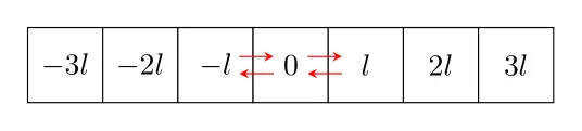
After sometime, the particle made some $k$ jumps to the right and the rest to the left , so the probability of finding this particle at position $x$ after $N$ jumps can be modeled accuretly by the binomial probability distribution function:
\[u(k,N) = {}^N C_k\; q^k(1-q)^{N-k}\] \[x = kl - (N-k)l \rightarrow k = \frac{1}{2}\left(N+\frac{x}{l}\right)\]According to central limit theorem : For large values of N $(>30)$ , the binomial distribution approaches the Gaussian (normal) distribution. To do so, we have to find two distinguishing characteristics of Gaussian distribution: mean and variance.
\[\langle x \rangle = \sum_{i=1}^{N} \langle x_i \rangle = N(ql-(1-q)l)\]Obviously, for the unbiased case, $\langle x \rangle = 0$
\[\sigma^2 = \langle x^2 \rangle - \langle x \rangle ^2 = 4Nl^2q(1-q)\]which simply yields:
\[u(x,N) \approx \frac{1}{\sigma\sqrt{2\pi}} \exp\left[-\frac{(x-\langle x \rangle)^2}{2\sigma^2}\right]\]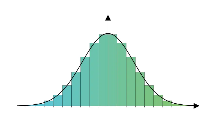
Numerical Solution
For the 1D case, the partial differential equation can be rewritten as :
\[\frac{\partial u}{\partial t} = D \;\frac{\partial^2 u }{\partial x^2}\]Finite Difference Method (FDM)
Mainly,there are 3 ways to compute derivatives numerically (forward scheme , backward scheme , central scheme). Considering a step size of value $h = \Delta x$ around $x$.
Forward Difference Scheme
With Taylor expansion, we get:
\[f(x+h) = \sum_{n=0}^{\infty} h^n \frac{f^{(n)}(x)}{n!} = f(x) + hf'(x) + h^2\frac{f''(x)}{2!} + h^3\frac{f'''(x)}{3!}+ ...\]Solving for $f’(x)$
\[f'(x) = \frac{1}{h}\left(f(x+h) - f(x) - h^2\frac{f''(x)}{2!} - h^3\frac{f'''(x)}{3!}- ... \right)\;\;\;\; \rightarrow (1)\] \[f'(x) = \frac{f(x+h) - f(x)}{h} +\mathcal{O}(h)\]Backward Difference Scheme
\[f(x-h) = \sum_{n=0}^{\infty} (-h)^n \frac{f^{(n)}(x)}{n!} = f(x) - hf'(x) + h^2\frac{f''(x)}{2!} - h^3\frac{f'''(x)}{3!}+ ...\]Solving for $f’(x)$
\[f'(x) = \frac{1}{h}\left(f(x) - f(x-h) + h^2\frac{f''(x)}{2!} - h^3\frac{f'''(x)}{3!}+ ... \right) \;\;\;\; \rightarrow (2)\] \[f'(x) = \frac{f(x) - f(x-h)}{h} +\mathcal{O}(h)\]Central Difference Scheme
Both forward and backward difference techniques have the same error which grows linearly with $h$… Can we do better ? Yeah , of course.
By adding equation $(1)$ and $(2)$, we have:
\[f'(x) = \frac{f(x+h) - f(x-h)}{2h} +E(h)\] \[E(h) = -h^2\frac{f'''(x)}{3!} - h^4\frac{f'''''(x)}{5!}-...\]which can be rewritten as :
\[f'(x) = \frac{f(x+h) - f(x-h)}{2h} +\mathcal{O}(h^2)\]since $ 0 < h < 1$, $\mathcal{O}(h^2)$ as an error is so small. So, central difference technique is much better than forward and backward difference.
Applying central difference technique to solve for $\frac{d^2f}{dx^2} $
\[\frac{d^2f}{dx^2} = \frac{f(x+h)-2f(x) +f(x-h)}{h^2}\]Discrete Solution
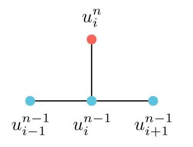
Using a 4-point stencil we can solve the 1D diffusion equation.
\[\frac{u_{i}^{n} - u_{i}^{n-1}}{\Delta t } = D \frac{u_{i+1} - 2u_i+u_{i-1}}{h^2}\] \[u_{i}^{n} = u_{i}^{n-1}+ D \Delta t \left(\frac{u_{i+1} - 2u_i+u_{i-1}}{h^2}\right)\]Note that $i$ is for spatial step in $x$ , while $n$ is for time step.
Simulation
Leveling up !
It is the time to solve the 2D Diffusion equation with nearly the same approach of the 1D case.
\[\frac{\partial u}{\partial t} = D \;\left(\frac{\partial^2 u }{\partial x^2} + \frac{\partial^2 u }{\partial y^2} \right)\]The generalized bi-variate Gaussian distribution function is given by:
\[u(x,y) = \frac{1}{2\pi\sigma_x\sigma_y\sqrt{1-\rho^2}} \exp{\left[-\frac{Z}{2(1-\rho^2)}\right]}\] \[Z = \frac{(x-\mu_x)^2}{\sigma_x^2}-\frac{2\rho(x-\mu_x)(y-\mu_y)}{\sigma_x\sigma_y}+\frac{(y-\mu_y)^2}{\sigma_y^2}\]where:
\[\rho = Cor(x,y) = \frac{\sigma_{xy}}{\sigma_x\sigma_y}\]Discrete Solution
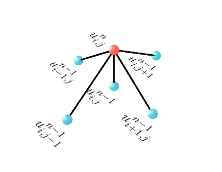
Similarly,using a 6-point stencil we can solve the 2D diffusion equation.
\[\frac{u_{i,j}^{n} - u_{i,j}^{n-1}}{\Delta t } = D\left(\frac{u_{i+1,j} - 2u_{i,j}+u_{i-1,j}}{\Delta x^2}+\frac{u_{i,j+1} - 2u_{i,j}+u_{i,j-1}}{\Delta y^2}\right)\] \[u_{i,j}^{n} = u_{i,j}^{n-1}+ D \Delta t \left(\frac{u_{i+1,j} - 2u_{i,j}+u_{i-1,j}}{\Delta x^2}+\frac{u_{i,j+1} - 2u_{i,j}+u_{i,j-1}}{\Delta y^2}\right)\]To make things more simple for us, we are going to set $\Delta x = \Delta y$
Again $i,j$ are for spatial steps in $x$ and $y$ , while $n$ is for time step.
Simulation
Now, it the time to head the real physical system and how it operates in the form of a brownian motion.
Brownian Motion
Brownian motion is a form of stochastic motion of particles induced by random collisions with surrounding fluid molecules combined with Diffusiophoresis you can get an approximate particle diffusion simulation. Diffusiophoresis is a spontaneous movement of the bulk of particles controlled by the concentration gradient. It also obeys the formula of approximated Gaussian density function we have derived. There are some simulation methods we can use to describe a Brownian Motion: Einstein-Smoluchowski’s, which treats the whole situation as a random walk model, and Langevin’s theory, which, on the other hand, involves a differential equation to describe the Brownian motion of the particles.
Einstein-Smoluchowski’s Theory
It is a fairly simple approach we can start with. we begin with a particle as a unitary example. So, the general relationship between the particle before and after $n$ random collisions can be formulated as:
\[r_n = r_{n-1} + S.k \;\;\; \rightarrow (3)\]where:
$r_n$ is the current position vector of the particle
$r_{n-1}$ is the pervious position vector of the particle
$S$ is the distance the particle moves after each collision (related to the Diffusion coefficient)
$k$ is a random movement vector
1D case
Assume that the particles moves along the x-axis, so the random movement vector $k$ can be expressed as :
\[k \in \{-1,1\} \;\;\; \rightarrow \;\;\; k_{1D} = k\hat{x}\]As we cannot build much of a intuition from a 1D simulation, we can ignore it.
2D case
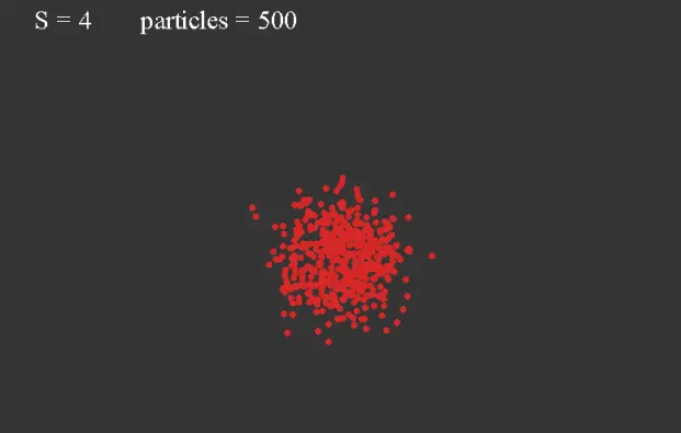
As opposed to the 1D case, the particle is free to move in all directions, so we better define a random angle parameter $\theta$. Note that in this case the generated random coordinates are uniformly distributed over the unit ring. Thus, $k$ , in this situation, is defined as:
\[\theta \in [0,2\pi] \;\;\; \rightarrow \;\;\; k_{2D} = \cos{\theta}\;\hat{x} + \sin{\theta}\;\hat{y}\]So, what we have to do is just adding some particles to the screen and let them spread out, but bare in mind that the internal forces of attraction and gravity are neglected in this model. The initial setup should look like this:
Jump to the Simulation (youtube video)
3D case
Now we have a bit of a trouble here generating random coordinates. The common way to do it is to use the parameters of the spherical coordinate $(\theta, \phi)$, but the randomized movement vector $k_{3D}$ will not be uniform over the surface of the unit sphere; however, the points will be more dense near the poles and sparse near the equator.
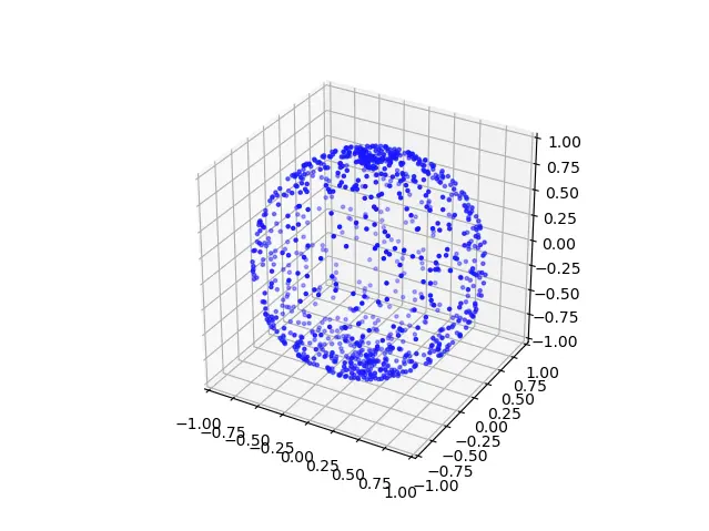
One way to do it is generating three random numbers $(a,b,c)$ and normalize them like so:
\[\alpha = \frac{a}{\sqrt{a^2+b^2+c^2}}\] \[\beta = \frac{b}{\sqrt{a^2+b^2+c^2}}\] \[\gamma = \frac{c}{\sqrt{a^2+b^2+c^2}}\]And, we shall get something like this- amazing, isn’t it ?
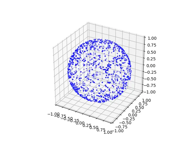
So, the movement vector $k_{3D}$ can be expressed as:
\[a ,b,c \in [-1,1] \;\;\; \rightarrow \;\;\; k_{3D} = \alpha\;\hat{x} + \beta\;\hat{y} + \gamma \;\hat{z}\]We can use this way in the 2D case, but the 2D randomization is already uniform, so we anticipate getting similar results.
Langevin Theory
This model is more accurate than Einstein-Smoluchowski’s model as it takes into account the forces act on the system, and also follows newton second law.
\[\sum F = m \frac{d^2r}{dt^2}\] \[-\alpha\frac{dr}{dt} + \eta(t) + F_{ext}(t) = m \frac{d^2r}{dt^2}\]where:
$\alpha\frac{dr}{dt}$ is the damping force.
$\eta(t)$ is noise term, or simply the impact of the internal collisions between the particles of the fluid.
$F_{ext}(t)$ represents the external forces act on the particles.
We are not going to dig further into Langevin model, but we might conclude that both random walk and Langevin hold and explicitly describe the system; nevertheless, radom walk is more suitable for many-particle system due to the efficient computations involved. On the other hand, Langevin is more appropriate in the case of single particle induced by number of forces, giving us a more of smooth trace.
References
Grant Sanderson video on diffusion equation